



MR_Lab_2_plot
ipynb316 kBPython · 28 cellsIn Lab 2: Plotting
Ploting
Jupyter notebooks
This is a space where text and code come together to form a coherent document. Throughout the course, we will make use of Jupyter notebooks for illustration purposes and for experimentation.
Plotting
Plotting is very useful to visualize data and can be easily done via the matplotlib library in Python. To perform some plotting, we need (at the very least) 2 lists X and Y that represent the x-coordinate and y-coordinate values, respectively. We also need to write one import statement, and we are all set.
Let's plot the function y = x^2 for x = 0, 1, 2, ... , 9. Using list-comprehension, we create the required lists:
import matplotlib.pyplot as plt

X = [i for i in range(0, 10)]
Y = [x**2 for x in X]

plt.plot(X, Y)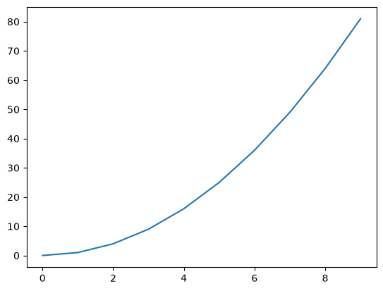
To customize our plot, we can invoke additional commands that take strings as inputs to display the x-labels, y-labels, and give our figure a title.
plt.plot(X, Y, color='g')
plt.xlabel("x")
plt.ylabel("f(x)")
plt.title("quadratic function")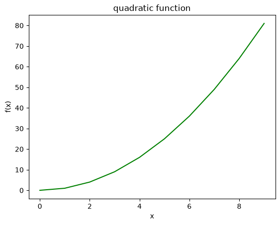
Refining the x-coordinate range
What if we need to plot y = x^2 in a small interval? Example, for 0 <= x <= 2. Using our usual method, we only have 3 data points:
X = [i for i in range(0, 3)]
Y = [x**2 for x in X]
plt.plot(X, Y, 'red')
plt.xlabel("x")
plt.ylabel("f(x)")
plt.title("quadratic function")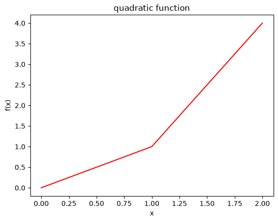
As you can observe from the figure, it is not smooth enough and unlike our expectation from the quadratic function. This is due to the fact that there is a small number of points used to plot and they are connected using straight-lines.
We can refine our x-coordinate list into many smaller points and then plot:
X = [0.01*i for i in range(0, 201)] # refined interval
Y = [x**2 for x in X]
plt.plot(X, Y, 'red')
plt.xlabel("x")
plt.ylabel("f(x)")
plt.title("quadratic function")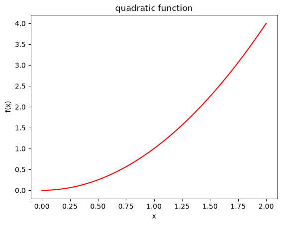
As can be seen, the above figure is more accurate.
Multiple plots on the same figure
Using the matplotlib.pyplot module, we can plot multiple graphs on the same figure. Typically, the figures have the same x-points list X and different y-values list. It is important in this case to use the label attribute in .plot() and then invoke the .legend() command to display these labels.
Example:
import matplotlib.pyplot as plt

X = [0.01*i for i in range(0, 201)]
Y = [x**2 for x in X]
Z = [x for x in X]

plt.plot(X, Y, color='r', label='quadratic')
plt.plot(X, Z, color='g', label='linear')
plt.xlabel("x")
plt.ylabel("y")
plt.title("Multiple plots")
plt.legend()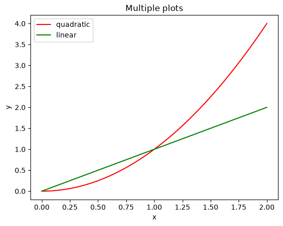
Subplots
Any figure can be split into rows and columns using plt.subplot(a, b, c):
a: is the parameter specifying the number of rowsb: is the parameter specifying the number of columnsc: is the parameter specifies the figure we're plotting out of the total subfigures In general, thecparameter moves from the left to the right, top to bottom.
It is a good idea to use the plt.figure(x) command before the plt.subplot() to
specify which figure we are splitting into subplits. For example, if we need 2 figures where: the first figure consists of 1 row and 2 columns:
a=1,b=2c=1is the left subplot,c=2is the right subplot
the second figure consists of 2 rows and 2 columns:
a=2,b=2c=1is the upper-left figure,c=2is the top-right figure,c=3is bottom-left, andc=4is the bottom-right figure.
Example:
import matplotlib.pyplot as plt

X = [0.01*i for i in range(0, 200)]
Y = [x**2 for x in X]
Z = [x for x in X]

# first figure (split into two horizontally)
plt.figure(1)
plt.subplot(1, 2, 1) # left figure
plt.plot(X, Y, color='r')
plt.xlabel("x")
plt.title("Subplot 1")

plt.subplot(1, 2, 2) # right figure
plt.plot(X, Z, color='g')
plt.xlabel("x")
plt.title("Subplot 2")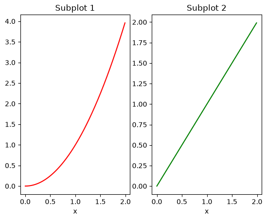
import matplotlib.pyplot as plt

X = [0.01*i for i in range(0, 200)]
Y = [x**2 for x in X]
Z = [x for x in X]


# second figure (split into 4)
plt.figure(2)
plt.subplot(2, 2, 1) # top-left figure
plt.plot(X, Y, color='r')
plt.xlabel("x")
plt.title("Subplot 1")

plt.subplot(2, 2, 2) # top-right figure
plt.plot(X, Z, color='g')
plt.xlabel("x")
plt.title("Subplot 2")

plt.subplot(2, 2, 3) # top-left figure
plt.plot(X, Y, color='b')
plt.xlabel("x")
plt.title("Subplot 3")

plt.subplot(2, 2, 4) # top-right figure
plt.plot(X, Z, color='k')
plt.xlabel("x")
plt.title("Subplot 4")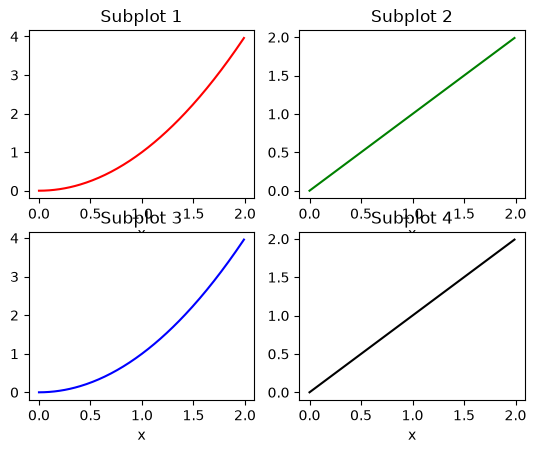
Histograms
A histogram is a diagram consisting of rectangles whose area is proportional
to the frequency of a variable and whose width is equal to the class interval. You can use the hist command in Python from the matplotlib package.
Example:
import matplotlib.pyplot as plt

data = [2, 1, 4, 3, 3, 6, 4, 2, 3]
plt.figure(3)
plt.hist(data, bins=len(data), facecolor='r', edgecolor='c')
plt.xlabel("data")
plt.ylabel("frequency")
plt.title("Histogram")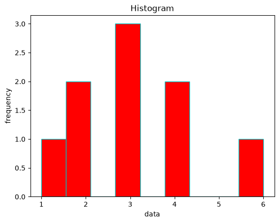
Bar Charts
We can use the plt.bar command to plot a bar-chart. Here, two lists are required: the x-coordinates list and heights list.
Example:
import matplotlib.pyplot as plt

left_edges = [0, 10, 20, 30, 40]
heights = [100, 200, 300, 400, 500]
plt.bar(left_edges, heights)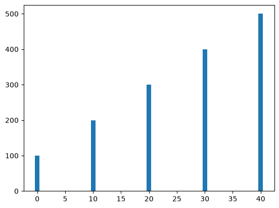
In the example: left_edges are the x-coordinates at which the bars will be drawn, and heights contains the lengths of bars for each coordinate in left_edges. The default width of each bar in a bar graph is 0.8 along the x-axis, which can be changed by passing a third argument to plt.bar.
plt.bar(left_edges, heights, 5)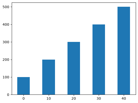
Pie Charts
We can use the plt.pie command to plot a pie-chart. Here, two lists are required: the labels list and sizes list.
import matplotlib.pyplot as plt

list_of_labels = ["Python", "C++", "Ruby", "Java"]
sizes = [200, 140, 250, 210]
plt.pie(sizes, labels=list_of_labels)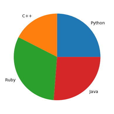
In the example, the sum of sizes list is 800. Accordingly, the label “Python” is assigned a pie slice of size 200/800, “C++” a pie slice of size 140/800, etc. There also optional keyword parameters for the plt.pie such as: colors, shadow, startangle.
plt.pie(sizes, labels=list_of_labels, shadow=True, startangle=120)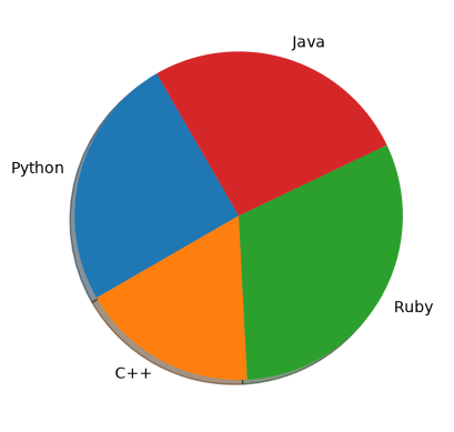
For more on the matplotlib.pyplot library, check the tutorial.