



MR_Lab_5_Pytorch_tutorial_Part2_A Gentle Introduction to torch.autograd
ipynb34 kBPython · 19 cellsIn Lab 5: Autograd
A Gentle Introduction to torch.autograd
torch.autograd is PyTorch’s automatic differentiation engine that powers
neural network training. In this section, you will get a conceptual
understanding of how autograd helps a neural network train.
When training neural networks, the most frequently used algorithm is back propagation. In this algorithm, parameters (model weights) are adjusted according to the gradient of the loss function with respect to the given parameter.
The gradient of the loss function with respect to a parameter is the partial derivative of the loss (rate of change) with respect to that specific parameter.
This gradient, a vector of these partial derivatives for all parameters, indicates the direction and rate of steepest ascent of the loss function's surface at the current parameter values. In practice, machine learning models use this gradient to adjust parameters in the opposite direction (steepest descent), thereby minimizing the loss and improving prediction accuracy.
Note: The derivative of a function gives the instantaneous rate of change of the function with respect to its input variable.
- If the function is descending, then the derivative is negative
- If the function is ascending, then the derivative is positive
To compute those gradients, PyTorch has a built-in differentiation engin: torch.autograd
.
It supports automatic computation of gradient for any computational graph.
Consider the simplest one-layer neural network, with input x, parameters w and b, and some loss function. It can be defined in PyTorch in the follo manner:ner:
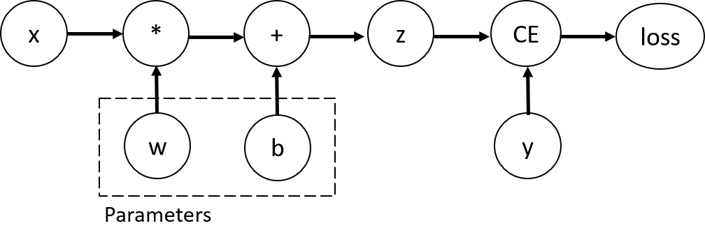
In this network, w and b are parameters, which we need to optimize. Thus, we need to be able to compute the gradients of loss function with respect to those variables. In order to do that, we set the requires_grad property of those tensors.
NOTE: You can set the value of requires_grad when creating a tensor, or later by using x.requires_grad_(True) method.
import torch
x = torch.ones(5)  # input tensor
y = torch.zeros(3)  # expected output
w = torch.randn(5, 3, requires_grad=True)
b = torch.randn(3, requires_grad=True)
z = torch.matmul(x, w)+b
loss = torch.nn.functional.binary_cross_entropy_with_logits(z, y) #Calculate Binary Cross Entropy between target and input logits.
print("x:", x , "\n")
print("w:", w, "\n")
print("b:", b, "\n")
print("z:",  z, "\n")

print("y:", y, "\n")
print("loss:", loss)
x: tensor([1., 1., 1., 1., 1.])
w: tensor([[ 0.2070, -0.9089, -0.7129],
[ 1.3084, -0.7705, 0.0434],
[-0.0649, -0.6241, -0.8535],
[ 0.4156, -0.1223, 0.5745],
[-0.0812, -0.8423, -0.8018]], requires_grad=True)
b: tensor([ 0.6392, 0.7339, -2.3566], requires_grad=True)
z: tensor([ 2.4241, -2.5343, -4.1069], grad_fn=<AddBackward0>)
y: tensor([0., 0., 0.])
loss: tensor(0.8672, grad_fn=<BinaryCrossEntropyWithLogitsBackward0>)
A function that we apply to tensors to construct computational graph is in fact an object of class Function.
This object knows how to compute the function in the forward direction, and also how to compute its derivative during the backward propagation step.
A reference to the backward propagation function is stored in grad_fn property of a tensor.
print(f"Gradient function for x = {x.grad_fn}")
print(f"Gradient function for y = {y.grad_fn}")
print(f"Gradient function for w = {w.grad_fn}")
print(f"Gradient function for b = {b.grad_fn}")
print(f"Gradient function for z = {z.grad_fn}")
print(f"Gradient function for loss = {loss.grad_fn}")
Gradient function for x = None Gradient function for y = None Gradient function for w = None Gradient function for b = None Gradient function for z = <AddBackward0 object at 0x000002D23ADC8100> Gradient function for loss = <BinaryCrossEntropyWithLogitsBackward0 object at 0x000002D23ADC8100>
Computing Gradients
To optimize weights of parameters in the neural network, we need to compute the derivatives of our loss function with respect to parameters, namely, we need and under some fixed values of x and y
when using loss.backward(), Backpropagation is applied. PyTorch's Automatic Differentiation Engine (autograd) traverses the computational graph backward.
Gradients are calculated using loss.backward(). It computes the partial derivatives of the loss with respect to any tensor with requires_grad=True.
Computing gradients only tells PyTorch the direction and rate of change. It does not update the actual weight and bias value
These gradients are stored in the .grad attribute of w and b (w.grad and b.grad)
the values of those derivatives can be retrieved from w.grad and b.grad
print("w:", w)
print("b:", b)
loss.backward() # backpropagation
print("w.grad:", w.grad)
print("b.grad:", b.grad)
print("w:", w) # w is not changed
print("b:", b) # b is not changed
w: tensor([[ 0.2070, -0.9089, -0.7129],
[ 1.3084, -0.7705, 0.0434],
[-0.0649, -0.6241, -0.8535],
[ 0.4156, -0.1223, 0.5745],
[-0.0812, -0.8423, -0.8018]], requires_grad=True)
b: tensor([ 0.6392, 0.7339, -2.3566], requires_grad=True)
w.grad: tensor([[0.3062, 0.0245, 0.0054],
[0.3062, 0.0245, 0.0054],
[0.3062, 0.0245, 0.0054],
[0.3062, 0.0245, 0.0054],
[0.3062, 0.0245, 0.0054]])
b.grad: tensor([0.3062, 0.0245, 0.0054])
w: tensor([[ 0.2070, -0.9089, -0.7129],
[ 1.3084, -0.7705, 0.0434],
[-0.0649, -0.6241, -0.8535],
[ 0.4156, -0.1223, 0.5745],
[-0.0812, -0.8423, -0.8018]], requires_grad=True)
b: tensor([ 0.6392, 0.7339, -2.3566], requires_grad=True)
NOTE
We can only obtain the grad properties for the leaf nodes of the computational graph, which have requires_grad property set to True.
For all other nodes in our graph, gradients will not be available.
We can only perform gradient calculations using backward once on a given graph, for performance reasons.
If we need to do several backward calls on the same graph, we need to pass retain_graph=True to the backward call.
How to change them?:
To actually update w and b using the calculated gradients, you need an optimizer (like torch.optim.SGD) and a step call:
print("w:", w)
print("b:", b)
optimizer = torch.optim.SGD([w, b], lr=0.001)
optimizer.step()  # This changes the values of w and b
print("w:", w) # w is changed
print("b:", b) # b is changed
w: tensor([[ 0.1733, -0.9116, -0.7135],
[ 1.2747, -0.7732, 0.0428],
[-0.0985, -0.6268, -0.8541],
[ 0.3819, -0.1250, 0.5739],
[-0.1149, -0.8450, -0.8024]], requires_grad=True)
b: tensor([ 0.6055, 0.7312, -2.3572], requires_grad=True)
w: tensor([[ 0.1730, -0.9116, -0.7135],
[ 1.2744, -0.7732, 0.0428],
[-0.0988, -0.6268, -0.8541],
[ 0.3816, -0.1250, 0.5739],
[-0.1152, -0.8450, -0.8024]], requires_grad=True)
b: tensor([ 0.6052, 0.7311, -2.3572], requires_grad=True)
Step-by-Step Parameter Update Breakdown
loss.backward(): Calculates how a tiny change in and affects the overall loss. This calculated gradient is automatically stored inw.gradandb.grad.- The Optimizer: Loops through every element of the parameters ( and ) individually to prepare for the update.
- The Value Update: Modifies the weights and biases by multiplying their stored gradients by the learning rate and subtracting that value from the current parameter state:
Disabling Gradient Tracking
By default, all tensors with requires_grad=True are tracking their computational history and support gradient computation.
However, there are some cases when we do not need to do that, for example, when we have trained the model and just want to apply it to some input data, i.e. we only want to do forward computations through the network.
We can stop tracking computations by surrounding our computation code with torch.no_grad() block:
z = torch.matmul(x, w)+b
print(z.requires_grad)

with torch.no_grad():
    z = torch.matmul(x, w)+b
print(z.requires_grad)
True False
let us try the forward and backward while freezing w (requires_grad=False)
import torch

x = torch.ones(5)  # input tensor
y = torch.zeros(3)  # expected output
w = torch.randn(5, 3, requires_grad=False) # Frozen
b = torch.randn(3, requires_grad=True)
z = torch.matmul(x, w)+b
loss = torch.nn.functional.binary_cross_entropy_with_logits(z, y) #Calculate Binary Cross Entropy between target and input logits.
loss.backward() # backpropagation

print("x:", x , "\n")
print("w:", w, "\n")
print("b:", b, "\n")
print("w.grad:", w.grad)
print("b.grad:", b.grad)
print("z:",  z, "\n")
print("y:", y, "\n")
print("loss:", loss)

optimizer = torch.optim.SGD([w, b], lr=0.01)
optimizer.step()  # This changes the values of w and b
print("w:", w) # w is not changed
print("b:", b) # b is changed
x: tensor([1., 1., 1., 1., 1.])
w: tensor([[-1.6166, -2.2661, -1.3580],
[ 0.3554, 0.8409, -0.2812],
[ 1.2156, -0.6953, 0.8419],
[ 1.7431, 1.5609, -0.6267],
[ 0.0282, 0.1363, -0.5562]])
b: tensor([-1.4987, 0.2442, -1.4946], requires_grad=True)
w.grad: None
b.grad: tensor([0.1855, 0.1518, 0.0100])
z: tensor([ 0.2270, -0.1791, -3.4746], grad_fn=<AddBackward0>)
y: tensor([0., 0., 0.])
loss: tensor(0.4837, grad_fn=<BinaryCrossEntropyWithLogitsBackward0>)
w: tensor([[-1.6166, -2.2661, -1.3580],
[ 0.3554, 0.8409, -0.2812],
[ 1.2156, -0.6953, 0.8419],
[ 1.7431, 1.5609, -0.6267],
[ 0.0282, 0.1363, -0.5562]])
b: tensor([-1.5006, 0.2427, -1.4947], requires_grad=True)