



MR_Lab_3_numpy
ipynb53 kBPython · 48 cellsIn Lab 3: NumPy
The numpy module
Introduction
Numpy is a Python package, it stands for numerical python. Using numpy we can perform operations such as:
- Mathematical and logical operations on arrays
- Operations related to linear algebra
- Built-in functions for random number generation
import numpy as npThe ndarray object
The most important object defined in NumPy is an N-dimensional array type called ndarray:
- It describes the collection of items of the same type
- Items in the collection can be accessed using a zero-based index
L = [1, 2, 3]
print(L)
a = np.array(L)
print(a)
[1, 2, 3] [1 2 3]
L = [[1, 2, 3], [4, 5, 6]]
a = np.array(L)
print(a)
[[1 2 3] [4 5 6]]
Computing the length of the array in numpy is done via the shape attribute:
print(a.shape)(2, 3)
Unlike Python lists, you can specify the data-type of the items in a numpy array. Python automatically casts all the items to the specified dtype. Once you specify the dtype, mixed types will not be allowed.
a_mixed = np.array([1, 'CSC243'])
print(a_mixed)
a_float = np.array([1, 2, 3 ], dtype=float)
print(a_float)
a_float = np.array([1.5, 2.7, 3.1 ], dtype=int)
print(a_float)
['1' 'CSC243'] [1. 2. 3.] [1 2 3]
Creating ndarray objects
Numpy ndarrays are created:
- As empty : empty function allocates memory without clearing it. The values inside will be arbitrary "garbage data" left over in your computer's RAM. You must overwrite them before reading from the array.
- As zeros
- As ones
- From existing data
a = np.empty((3,4), dtype=float)
print(a)
a = np.zeros((2,4))
print(a)
a = np.ones((3,2))
print(a)
a = np.ones((3,), dtype=int)
print(a)
[[0. 0. 0. 0.] [0. 0. 0. 0.] [0. 0. 0. 0.]] [[0. 0. 0. 0.] [0. 0. 0. 0.]] [[1. 1.] [1. 1.] [1. 1.]] [1 1 1]
Ranges
You can create ranges of data through:
np.arange(start, stop, step, dtype): returns anndarrayobject containing evenly spaced values within a given range.np.arange(stop, dtype): returns anndarrayobject containing evenly spaced values from 0 till stop-1.np.linspace(start, stop, num, dtype): instead of step size, the number num of evenly spaced values in the interval is specified.
r = np.arange(1.5, 2, 0.1)
print(r)
r = np.arange(5)
print(r)
r = np.linspace(10, 50, 5)
print(r)
[1.5 1.6 1.7 1.8 1.9] [0 1 2 3 4] [10. 20. 30. 40. 50.]
One advantage of using numpy.arange instead of range is that the step-size can
be of type float in this case.
Math functions using numpy
Mathematical functions can also be accessed from the numpy module (sin,
cos, exp, ceil, floor, etc.). The advantage of using numpy functions is that we can pass a full array as an input (in contrast to the functions from the math module, which take a single value as input).
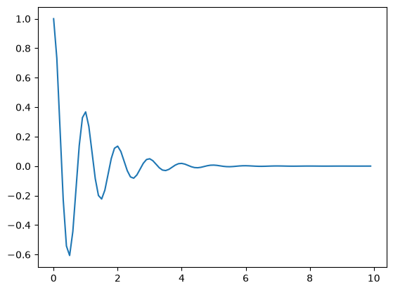
Example: plotting exp(-x)*cos(2πx), for x = [0, 0.1, 0.2, …, 9.9]
from math import pi
import matplotlib.pyplot as plt

X = np.arange(0, 10, 0.1)
Y = np.exp(-X)*np.cos(2*pi*X)
print(Y)
plt.plot(X, Y)
[ 1.00000000e+00 7.32028848e-01 2.53001717e-01 -2.28925420e-01 -5.42300309e-01 -6.06530660e-01 -4.43997940e-01 -1.53453298e-01 1.38850286e-01 3.28921764e-01 3.67879441e-01 2.69298364e-01 9.30741301e-02 -8.42169556e-02 -1.99501135e-01 -2.23130160e-01 -1.63337714e-01 -5.64523135e-02 5.10801656e-02 1.21003555e-01 1.35335283e-01 9.90693315e-02 3.42400590e-02 -3.09816865e-02 -7.33923659e-02 -8.20849986e-02 -6.00885870e-02 -2.07676456e-02 1.87913428e-02 4.45147201e-02 4.97870684e-02 3.64455703e-02 1.25962138e-02 -1.13975255e-02 -2.69995426e-02 -3.01973834e-02 -2.21053558e-02 -7.63998984e-03 6.91294868e-03 1.63760504e-02 1.83156389e-02 1.34075760e-02 4.63388808e-03 -4.19291532e-03 -9.93257663e-03 -1.11089965e-02 -8.13210594e-03 -2.81059519e-03 2.54313170e-03 6.02441225e-03 6.73794700e-03 4.93237158e-03 1.70471216e-03 -1.54248735e-03 -3.65399074e-03 -4.08677144e-03 -2.99163459e-03 -1.03396019e-03 9.35565868e-04 2.21625741e-03 2.47875218e-03 1.81451810e-03 6.27128556e-04 -5.67449383e-04 -1.34422807e-03 -1.50343919e-03 -1.10056086e-03 -3.80372697e-04 3.44175449e-04 8.15315539e-04 9.11881966e-04 6.67523905e-04 2.30707703e-04 -2.08752962e-04 -4.94513872e-04 -5.53084370e-04 -4.04873715e-04 -1.39931295e-04 1.26615072e-04 2.99937825e-04 3.35462628e-04 2.45568321e-04 8.48726207e-05 -7.67959230e-05 -1.81921487e-04 -2.03468369e-04 -1.48944716e-04 -5.14778466e-05 4.65790818e-05 1.10340959e-04 1.23409804e-04 9.03395368e-05 3.12228923e-05 -2.82516412e-05 -6.69251749e-05 -7.48518299e-05 -5.47936988e-05 -1.89376414e-05 1.71354866e-05 4.05921705e-05]
Statistical Operations
We can compute the minimum and maximum through np.amin(a, axis=) and np.amax(a, axis=). The axis keyword specifies the dimension over which min/max is computed. If not specified, the min/max will be computed over the whole array.
a = np.array([[7,2], [3,4], [5,6]])
print("a =\n" + str(a))
print("min:", np.amin(a))
print("minima (axis=0):", np.amin(a, axis=0))
print("minima (axis=1):", np.amin(a, axis=1))
a = [[7 2] [3 4] [5 6]] min: 2 minima (axis=0): [3 2] minima (axis=1): [2 3 5]
We can also compute the average (mean), median, standard deviation and variance. We use in these cases np.mean(), np.median(), np.std(), and np.var(), respectively. All these functions also admit an axis keyword parameter like np.amin.
Generation Random Numbers
We can generate random numbers using numpy.random. Here are a few examples:
import numpy.random as rand

x = rand.uniform(1, 10)
print(x)
8.323015843186308
The random.uniform(x, y) function generates a uniformly-distributed random float in the real interval [x, y]. The default values are x=0, y=1.
The random.randint generates a random integer between a and b inclusive.
Multiple runs of the same code give different random numbers (that is whole point).
a = np.random.randint(3,500)
print("a=",a)
a= 263
a = 1
b = 5
y = rand.randint(a, b+1)
print(y)
3
arrayD = np.random.randint(3,500,10)
print(arrayD.shape)
print ("arrayD=" , arrayD)
(10,) arrayD= [253 378 103 420 65 180 88 181 388 141]
Pseudo-random values
Numpy can be used to generate pseudo-random values from various distributions.
In particular, a very useful distribution is the standard normal (zero mean and unit variance).
Let's generate two vectors sampled from the normal distribution, using a length parameter that we'll be able to change if needed.
The numpy.random.randn() function in Python's NumPy library is used to generate random numbers sampled from the standard normal distribution.
length = 50

vecA = np.random.randn(length)
vecB = np.random.randn(2*length)

print("vecA:" , vecA)
print("vecB:" , vecB)
vecA: [-2.10999809 -2.11287348 1.25280955 -0.4924122 -0.2719082 -0.46451978 -0.64062689 0.19295273 -0.41339376 -0.3080825 -0.83406057 0.64042542 0.33229005 1.14290607 1.32707561 -0.51302455 0.97914793 1.91572189 -1.69386572 -1.49945308 -0.9944069 0.06943031 -1.06752387 -0.39937929 1.99114138 -0.1341258 -0.80091109 2.10253385 1.35524086 -1.58320581 0.93282241 0.92543729 1.09713833 -1.44882033 -0.69751291 -0.36215201 -0.88251173 0.07514971 -0.25168008 -1.36534188 -1.66889414 0.32727418 -0.13753305 1.0402394 -1.03755714 -0.45327112 -0.48093412 -1.0695069 0.93856271 -1.81933384] vecB: [ 0.61000751 0.74915139 0.45793863 1.32809655 0.95842044 0.80711744 -0.22509216 -0.13273978 0.22428596 -0.41573978 -1.12103327 1.55300499 1.03583227 -0.30461149 -0.97857771 -0.41309167 -2.17345279 -0.20978699 0.23694952 0.64353891 0.27651094 0.60680622 -0.38087215 1.7829058 -0.30146565 2.00674765 0.37022398 -0.7213519 1.06728759 0.13603953 1.08551771 -0.09959652 -1.68196758 -1.14129733 -2.01333562 -0.38119678 -0.88047318 0.2568253 0.01893283 -0.64069811 -0.05745972 0.24583993 -0.73779167 0.83560195 -0.14166213 -0.29284934 -1.12737178 0.02145714 -0.92795249 0.006617 0.57357712 -1.54218791 0.40486226 0.19323385 0.011521 -0.39188825 0.73097972 1.0469983 1.24918161 1.57031582 -1.32300042 -0.78927998 0.57348572 -0.24271261 -0.83282858 0.06148128 -0.85546067 -0.31907881 -0.13937268 1.57481757 -0.05967344 0.70178645 1.19600514 0.21307818 -1.13968704 -1.24644357 -0.15612841 -0.14511488 -0.26215745 0.49376606 -0.057528 0.29816377 0.15734146 0.97027566 2.2217015 0.4296192 0.07338254 -0.04901035 -0.42025307 -1.49786917 -0.92738247 0.19970072 -0.96130874 -1.35304152 -0.20948683 -0.3770746 0.04890955 -0.8281197 0.54528106 -0.26623394]
vecA and vecB are numpy arrays. One of their attributes can be fetched to check their shape
print(vecA.shape)
print(vecB.shape)
(50,) (100,)
Numpy arrays can be vectors as well as matrices, or any tensor. For example the following code will create tensors with 3 dimensions using the standard normal
arrayC = np.random.randn(3,10,4)
print(arrayC.shape)
print(arrayC)
(3, 10, 4) [[[ 0.6103493 -0.9977386 1.24149819 0.59300844] [-0.73872367 0.60845882 0.28568399 -0.43267838] [-1.00679062 0.83438667 -0.80427253 -1.36078233] [ 0.44765166 2.14543953 -1.16122586 0.35655495] [ 0.25315243 0.86576808 -0.57761026 -0.73250677] [-2.85917571 1.13342275 0.01235514 0.42349046] [-0.71878794 -0.30369568 0.37075242 0.05745539] [ 0.02791402 0.41983534 -1.00716576 1.34233683] [-0.0413135 -1.41137134 -0.02696279 1.39171478] [ 0.331664 -0.79183008 1.77118333 -1.44127238]] [[-1.38259346 -0.96248992 -0.24504574 0.08487525] [ 2.50138512 -1.10035743 -0.60987928 0.040802 ] [-0.84004769 -1.55645974 1.43365243 -1.2556008 ] [ 0.78793701 -1.96177205 -3.01223948 -0.50406417] [ 0.2043025 0.39563536 -0.75635317 0.67337065] [-0.22398293 -0.50307142 1.15947818 0.0841907 ] [ 0.24221879 -0.66059901 -1.38996028 -1.62408543] [ 0.0883038 1.36255269 -2.08206203 0.24684805] [ 1.54575432 1.18894425 0.08715927 1.08013783] [ 1.42112677 1.09184144 0.48053391 0.09083689]] [[ 0.55342773 1.52352332 0.66681621 0.80510851] [-0.85783124 0.46091983 -0.25287231 1.98495604] [ 0.64906538 -2.03134777 0.74839709 -0.68752474] [ 1.05048703 0.66923679 1.52298283 -1.43924225] [-1.2473455 -0.94141396 -0.22155136 -0.57578813] [-0.92528658 1.06919995 2.54984813 -0.47304496] [-1.39855088 -0.75347335 -0.64908361 1.25573668] [ 2.02022871 -1.39817262 0.0887552 -0.12159651] [ 2.76382791 0.55718271 -0.21643165 0.03328396] [-1.82241942 0.48814035 -0.95816279 -1.60424608]]]
A very important features of arrays is the fact they can be used as iterables. For example, you can iterate over the dimensions of an array by simply "looping" over it using a for loop
for dim in arrayC:
    print(dim.shape)
(10, 4) (10, 4) (10, 4)
Also possible to enumerate along the dimension in order to get the index of the current "smaller" array
print('Initial shape is %d %d %d' % (arrayC.shape[0],arrayC.shape[1],arrayC.shape[2]))
print('Iterating over the first dimension using an index k')
for k,curdim in enumerate(arrayC):
    print('k = %d, shape is %d %d' % (k,curdim.shape[0],curdim.shape[1]))
Initial shape is 3 10 4 Iterating over the first dimension using an index k k = 0, shape is 10 4 k = 1, shape is 10 4 k = 2, shape is 10 4
Another important operation when working with Numpy Arrays is reshaping. Essentially, reshaping consists in changing the organisation of the array (in terms of dimension), while keeping the same number of elements. For example, a 20x10 2D array can be converted into a 4x5x10 array
A = np.random.randint(1,50,(10,20))
print('Initial shape of A is %d x %d' % (A.shape[0],A.shape[1]))
print(A)
B = A.reshape((4,5,10))
print('B is A reshaped to %d x %d x %d' % (B.shape[0],B.shape[1],B.shape[2]))
print(B)
Initial shape of A is 10 x 20 [[13 25 31 17 34 15 48 41 38 26 43 38 37 4 36 21 45 34 37 35] [ 8 26 36 21 28 14 19 47 34 31 20 37 26 3 20 7 40 19 32 44] [48 6 44 7 45 9 1 16 12 9 16 24 30 15 34 14 15 2 14 28] [ 7 3 5 26 30 38 8 43 25 4 36 6 9 43 18 31 10 13 26 26] [33 47 43 28 12 32 14 31 34 4 16 35 25 41 22 1 41 36 31 5] [13 12 6 10 25 16 19 34 9 24 22 4 19 29 29 25 38 8 35 26] [30 28 25 23 27 43 49 47 24 27 34 23 1 48 5 19 26 22 34 47] [41 12 25 39 37 9 22 7 2 15 11 24 40 24 23 40 21 14 26 4] [37 10 5 37 34 1 9 8 17 8 8 25 18 39 1 41 14 44 44 2] [31 15 19 38 44 31 31 6 36 23 14 4 48 36 32 23 47 27 48 12]] B is A reshaped to 4 x 5 x 10 [[[13 25 31 17 34 15 48 41 38 26] [43 38 37 4 36 21 45 34 37 35] [ 8 26 36 21 28 14 19 47 34 31] [20 37 26 3 20 7 40 19 32 44] [48 6 44 7 45 9 1 16 12 9]] [[16 24 30 15 34 14 15 2 14 28] [ 7 3 5 26 30 38 8 43 25 4] [36 6 9 43 18 31 10 13 26 26] [33 47 43 28 12 32 14 31 34 4] [16 35 25 41 22 1 41 36 31 5]] [[13 12 6 10 25 16 19 34 9 24] [22 4 19 29 29 25 38 8 35 26] [30 28 25 23 27 43 49 47 24 27] [34 23 1 48 5 19 26 22 34 47] [41 12 25 39 37 9 22 7 2 15]] [[11 24 40 24 23 40 21 14 26 4] [37 10 5 37 34 1 9 8 17 8] [ 8 25 18 39 1 41 14 44 44 2] [31 15 19 38 44 31 31 6 36 23] [14 4 48 36 32 23 47 27 48 12]]]
One property of numpy that is really important is broadcasting. The goal of broadcasting is to simplify the vectorization of certain operations when the vectors do not have the same shape. For example you can easily perform element-wise multiplication.
x = np.array([2,3])
y = np.array([[4,1],[9,10],[12,13]])
result = x*y
print("X: ",x)
print("Y: ")
print(y)
print("X shape is: ",x.shape)
print("Y shape is: ",y.shape)
print("Element-wise multiplication shape:", result.shape)
print("Element-wise multiplication result:")
print(result)
X: [2 3] Y: [[ 4 1] [ 9 10] [12 13]] X shape is: (2,) Y shape is: (3, 2) Element-wise multiplication shape: (3, 2) Element-wise multiplication result: [[ 8 3] [18 30] [24 39]]
Another very powerful tool in numpy is indexing. You can use either an integer vector or a boolean vector to choose which indexes you want to extract from your numpy tensor.
Consider that we want to extract all elements from the first line of your vector y that have a higher value than 1, you would have to do:
first_row = y[0]
print(first_row)
first_row_higher_than_one = first_row > 1
print("Result: ", first_row[first_row_higher_than_one])
[4 1] Result: [4]
You can also choose specific lines to query, for example if you want to query lines 0 and 2
rows = [0,2]
rows_result = y[rows]
values_higher_than_one = rows_result > 1
print("Result: ", rows_result[values_higher_than_one])
Result: [ 4 12 13]
You can also save and load your numpy tensors using np.savez and np.load. This will be really important in the next courses as this enable you to generate your data only once instead of having to do all the calculations every time you need your data.
filename = "y.npz"
source_tensor = y
np.savez(filename,data=source_tensor)loaded_npz = np.load(filename)
loaded_tensor = loaded_npz["data"]
print("Your tensor was loaded and contains: ", loaded_tensor)Your tensor was loaded and contains: [[ 4 1] [ 9 10] [12 13]]