MR_Lab_7_Pytorch_tutorial_Part4_NeuralNetwork
ipynb202 kBPython · 69 cellsIn Lab 7: Neural networks
Neural Networks
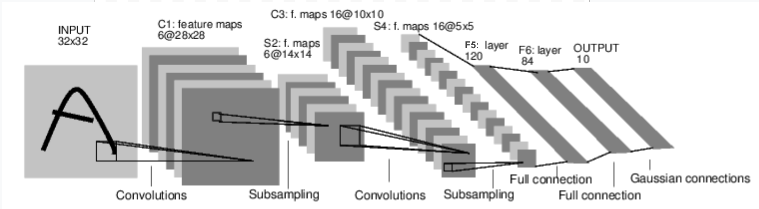
A typical training procedure for a neural network is as follows:
- Define the neural network that has some learnable parameters (or weights)
- Iterate over a dataset of inputs
- Process input through the network
- Compute the loss (how far is the output from being correct)
- Propagate gradients back into the network’s parameters
- Update the weights of the network, typically using a simple update rule:
\begin{align}weight = weight - learningRate * gradient\end{align}
Define the network
Let’s define this network:
import torch
import torch.nn as nn
import torch.nn.functional as F
print(torch.__version__)
2.14.0
We want to be able to train our model on a hardware accelerator like the GPU or MPS, if available.
Let’s check to see if torch.cuda or torch.backends.mps are available, otherwise we use the CPU.
device = (
    "cuda"
    if torch.cuda.is_available()
    else "mps"
    if torch.backends.mps.is_available()
    else "cpu"
)
print(f"Using {device} device")
Using mps device
NN Components
let us examine the component layers of NN
Module
nn.Module?[31mInit signature:[39m nn.Module(*args: Any, **kwargs: Any) -> [38;5;28;01mNone[39;00m
[31mDocstring:[39m
Base class for all neural network modules.
Your models should also subclass this class.
Modules can also contain other Modules, allowing them to be nested in
a tree structure. You can assign the submodules as regular attributes::
import torch.nn as nn
import torch.nn.functional as F
class Model(nn.Module):
def __init__(self) -> None:
super().__init__()
self.conv1 = nn.Conv2d(1, 20, 5)
self.conv2 = nn.Conv2d(20, 20, 5)
def forward(self, x):
x = F.relu(self.conv1(x))
return F.relu(self.conv2(x))
Submodules assigned in this way will be registered, and will also have their
parameters converted when you call :meth:`to`, etc.
.. note::
As per the example above, an ``__init__()`` call to the parent class
must be made before assignment on the child.
:ivar training: Boolean represents whether this module is in training or
evaluation mode.
:vartype training: bool
[31mInit docstring:[39m Initialize internal Module state, shared by both nn.Module and ScriptModule.
[31mFile:[39m ~/Desktop/Uni/LU-M2-AIDE/AIDE500- AI Programming Techniques/.venv/lib/python3.12/site-packages/torch/nn/modules/module.py
[31mType:[39m type
[31mSubclasses:[39m Identity, Linear, Bilinear, Threshold, ReLU, RReLU, Hardtanh, Sigmoid, Hardsigmoid, Tanh, ...Layers
Linear
nn.Linear??[31mInit signature:[39m
nn.Linear(
in_features: int,
out_features: int,
bias: bool = [38;5;28;01mTrue[39;00m,
device=[38;5;28;01mNone[39;00m,
dtype=[38;5;28;01mNone[39;00m,
) -> [38;5;28;01mNone[39;00m
[31mSource:[39m
[38;5;28;01mclass[39;00m Linear(Module):
[33mr"""Applies an affine linear transformation to the incoming data: :math:`y = xA^T + b`.[39m
[33m This module supports :ref:`TensorFloat32<tf32_on_ampere>`.[39m
[33m On certain ROCm devices, when using float16 inputs this module will use :ref:`different precision<fp16_on_mi200>` for backward.[39m
[33m Args:[39m
[33m in_features: size of each input sample[39m
[33m out_features: size of each output sample[39m
[33m bias: If set to ``False``, the layer will not learn an additive bias.[39m
[33m Default: ``True``[39m
[33m Shape:[39m
[33m - Input: :math:`(*, H_\text{in})` where :math:`*` means any number of[39m
[33m dimensions including none and :math:`H_\text{in} = \text{in\_features}`.[39m
[33m - Output: :math:`(*, H_\text{out})` where all but the last dimension[39m
[33m are the same shape as the input and :math:`H_\text{out} = \text{out\_features}`.[39m
[33m Attributes:[39m
[33m weight: the learnable weights of the module of shape[39m
[33m :math:`(\text{out\_features}, \text{in\_features})`. The values are[39m
[33m initialized from :math:`\mathcal{U}(-\sqrt{k}, \sqrt{k})`, where[39m
[33m :math:`k = \frac{1}{\text{in\_features}}`[39m
[33m bias: the learnable bias of the module of shape :math:`(\text{out\_features})`.[39m
[33m If :attr:`bias` is ``True``, the values are initialized from[39m
[33m :math:`\mathcal{U}(-\sqrt{k}, \sqrt{k})` where[39m
[33m :math:`k = \frac{1}{\text{in\_features}}`[39m
[33m Examples::[39m
[33m >>> m = nn.Linear(20, 30)[39m
[33m >>> input = torch.randn(128, 20)[39m
[33m >>> output = m(input)[39m
[33m >>> print(output.size())[39m
[33m torch.Size([128, 30])[39m
[33m """[39m
__constants__ = [[33m"in_features"[39m, [33m"out_features"[39m]
in_features: int
out_features: int
weight: Tensor
[38;5;28;01mdef[39;00m __init__(
self,
in_features: int,
out_features: int,
bias: bool = [38;5;28;01mTrue[39;00m,
device=[38;5;28;01mNone[39;00m,
dtype=[38;5;28;01mNone[39;00m,
) -> [38;5;28;01mNone[39;00m:
factory_kwargs = {[33m"device"[39m: device, [33m"dtype"[39m: dtype}
super().__init__()
self.in_features = in_features
self.out_features = out_features
self.weight = Parameter(
torch.empty((out_features, in_features), **factory_kwargs)
)
[38;5;28;01mif[39;00m bias:
self.bias = Parameter(torch.empty(out_features, **factory_kwargs))
[38;5;28;01melse[39;00m:
self.register_parameter([33m"bias"[39m, [38;5;28;01mNone[39;00m)
self.reset_parameters()
[38;5;28;01mdef[39;00m reset_parameters(self) -> [38;5;28;01mNone[39;00m:
[33m"""[39m
[33m Resets parameters based on their initialization used in ``__init__``.[39m
[33m """[39m
[38;5;66;03m# Setting a=sqrt(5) in kaiming_uniform is the same as initializing with[39;00m
[38;5;66;03m# uniform(-1/sqrt(in_features), 1/sqrt(in_features)). For details, see[39;00m
[38;5;66;03m# https://github.com/pytorch/pytorch/issues/57109[39;00m
init.kaiming_uniform_(self.weight, a=math.sqrt([32m5[39m))
[38;5;28;01mif[39;00m self.bias [38;5;28;01mis[39;00m [38;5;28;01mnot[39;00m [38;5;28;01mNone[39;00m:
fan_in, _ = init._calculate_fan_in_and_fan_out(self.weight)
bound = [32m1[39m / math.sqrt(fan_in) [38;5;28;01mif[39;00m fan_in > [32m0[39m [38;5;28;01melse[39;00m [32m0[39m
init.uniform_(self.bias, -bound, bound)
[38;5;28;01mdef[39;00m forward(self, input: Tensor) -> Tensor:
[33m"""[39m
[33m Runs the forward pass.[39m
[33m """[39m
[38;5;28;01mreturn[39;00m F.linear(input, self.weight, self.bias)
[38;5;28;01mdef[39;00m extra_repr(self) -> str:
[33m"""[39m
[33m Return the extra representation of the module.[39m
[33m """[39m
[38;5;28;01mreturn[39;00m f"in_features={self.in_features}, out_features={self.out_features}, bias={self.bias [38;5;28;01mis[39;00m [38;5;28;01mnot[39;00m [38;5;28;01mNone[39;00m}"
[31mFile:[39m ~/Desktop/Uni/LU-M2-AIDE/AIDE500- AI Programming Techniques/.venv/lib/python3.12/site-packages/torch/nn/modules/linear.py
[31mType:[39m type
[31mSubclasses:[39m NonDynamicallyQuantizableLinear, LazyLinear, Linear, LinearBn1d, Lineartorch.empty() is a PyTorch function that returns a tensor filled with uninitialized data.
This means that memory is allocated for the tensor, but its values are not set to any specific initial state (like zeros or random numbers).
The content of an empty tensor will be whatever data was already present in the allocated memory block before it was assigned to the tensor.
torch.empty?[31mDocstring:[39m
empty(*size, *, out=None, dtype=None, layout=torch.strided, device=None, requires_grad=False, pin_memory=False, memory_format=torch.contiguous_format) -> Tensor
Returns a tensor filled with uninitialized data. The shape of the tensor is
defined by the variable argument :attr:`size`.
.. note::
If :func:`torch.use_deterministic_algorithms()` and
:attr:`torch.utils.deterministic.fill_uninitialized_memory` are both set to
``True``, the output tensor is initialized to prevent any possible
nondeterministic behavior from using the data as an input to an operation.
Floating point and complex tensors are filled with NaN, and integer tensors
are filled with the maximum value.
Args:
size (int...): a sequence of integers defining the shape of the output tensor.
Can be a variable number of arguments or a collection like a list or tuple.
Keyword args:
out (Tensor, optional): the output tensor.
dtype (:class:`torch.dtype`, optional): the desired data type of returned tensor.
Default: if ``None``, uses a global default (see :func:`torch.set_default_dtype`).
layout (:class:`torch.layout`, optional): the desired layout of returned Tensor.
Default: ``torch.strided``.
device (:class:`torch.device`, optional): the desired device of returned tensor.
Default: if ``None``, uses the current device for the default tensor type
(see :func:`torch.set_default_device`). :attr:`device` will be the CPU
for CPU tensor types and the current CUDA device for CUDA tensor types.
requires_grad (bool, optional): If autograd should record operations on the
returned tensor. Default: ``False``.
pin_memory (bool, optional): If set, returned tensor would be allocated in
the pinned memory. Works only for CPU tensors. Default: ``False``.
memory_format (:class:`torch.memory_format`, optional): the desired memory format of
returned Tensor. Default: ``torch.contiguous_format``.
Example::
>>> torch.empty((2,3), dtype=torch.int64)
tensor([[ 9.4064e+13, 2.8000e+01, 9.3493e+13],
[ 7.5751e+18, 7.1428e+18, 7.5955e+18]])
[31mType:[39m builtin_function_or_methodprint(torch.empty(2,3))tensor([[0., 0., 0.],
[0., 0., 0.]])
torch.nn.Parameter?[31mInit signature:[39m torch.nn.Parameter(data=[38;5;28;01mNone[39;00m, requires_grad=[38;5;28;01mTrue[39;00m)
[31mDocstring:[39m
A kind of Tensor that is to be considered a module parameter.
Parameters are :class:`~torch.Tensor` subclasses, that have a
very special property when used with :class:`Module` s - when they're
assigned as Module attributes they are automatically added to the list of
its parameters, and will appear e.g. in :meth:`~Module.parameters` iterator.
Assigning a Tensor doesn't have such effect. This is because one might
want to cache some temporary state, like last hidden state of the RNN, in
the model. If there was no such class as :class:`Parameter`, these
temporaries would get registered too.
Args:
data (Tensor): parameter tensor.
requires_grad (bool, optional): if the parameter requires gradient. Note that
the torch.no_grad() context does NOT affect the default behavior of
Parameter creation--the Parameter will still have `requires_grad=True` in
:class:`~no_grad` mode. See :ref:`locally-disable-grad-doc` for more
details. Default: `True`
[31mFile:[39m ~/Desktop/Uni/LU-M2-AIDE/AIDE500- AI Programming Techniques/.venv/lib/python3.12/site-packages/torch/nn/parameter.py
[31mType:[39m _ParameterMeta
[31mSubclasses:[39m UninitializedParameterNotice in nn.Parameter the default requires_grad=True
Example on Linear:
input = torch.rand(3,2,4) # C x H x W
print("input:")
print(input)

LinearLayer=nn.Linear(in_features=4, out_features=3, bias=True)

print("\n Linear:")
print(LinearLayer)

print("\n LinearLayer weights:")
print(LinearLayer.weight)

print("\n bias:")
print(LinearLayer.bias)

out = LinearLayer(input)
print(out.size())
print("out:")
print(out)
input:
tensor([[[0.9983, 0.0532, 0.3933, 0.3754],
[0.5036, 0.7787, 0.9778, 0.6758]],
[[0.7831, 0.6580, 0.0144, 0.8392],
[0.4474, 0.7130, 0.4324, 0.4506]],
[[0.7834, 0.8924, 0.3921, 0.3244],
[0.0312, 0.9178, 0.6189, 0.8663]]])
Linear:
Linear(in_features=4, out_features=3, bias=True)
LinearLayer weights:
Parameter containing:
tensor([[-0.1356, 0.3215, 0.1471, -0.0642],
[ 0.2079, 0.3854, -0.3658, -0.1667],
[-0.1901, 0.2691, -0.0392, -0.4352]], requires_grad=True)
bias:
Parameter containing:
tensor([-0.1978, 0.2823, 0.0146], requires_grad=True)
torch.Size([3, 2, 3])
out:
tensor([[[-0.2824, 0.3040, -0.3397],
[ 0.0847, 0.2168, -0.2040]],
[[-0.1442, 0.5536, -0.3230],
[ 0.0054, 0.4169, -0.0916]],
[[ 0.0197, 0.5917, -0.0507],
[ 0.1285, 0.2718, -0.1456]]], grad_fn=<ViewBackward0>)
Convolutional Layer
nn.Conv2d?[31mInit signature:[39m
nn.Conv2d(
in_channels: int,
out_channels: int,
kernel_size: Union[int, tuple[int, int]],
stride: Union[int, tuple[int, int]] = [32m1[39m,
padding: Union[str, int, tuple[int, int]] = [32m0[39m,
dilation: Union[int, tuple[int, int]] = [32m1[39m,
groups: int = [32m1[39m,
bias: bool = [38;5;28;01mTrue[39;00m,
padding_mode: Literal[[33m'zeros'[39m, [33m'reflect'[39m, [33m'replicate'[39m, [33m'circular'[39m] = [33m'zeros'[39m,
device=[38;5;28;01mNone[39;00m,
dtype=[38;5;28;01mNone[39;00m,
) -> [38;5;28;01mNone[39;00m
[31mDocstring:[39m
Applies a 2D convolution over an input signal composed of several input
planes.
In the simplest case, the output value of the layer with input size
:math:`(N, C_{\text{in}}, H, W)` and output :math:`(N, C_{\text{out}}, H_{\text{out}}, W_{\text{out}})`
can be precisely described as:
.. math::
\text{out}(N_i, C_{\text{out}_j}) = \text{bias}(C_{\text{out}_j}) +
\sum_{k = 0}^{C_{\text{in}} - 1} \text{weight}(C_{\text{out}_j}, k) \star \text{input}(N_i, k)
where :math:`\star` is the valid 2D `cross-correlation`_ operator,
:math:`N` is a batch size, :math:`C_{\text{in}}` and :math:`C_{\text{out}}` correspond to
:attr:`in_channels` and :attr:`out_channels` respectively,
:math:`H` and :math:`W` are the input height and width in pixels.
See the Shape section below for how :math:`H_{\text{out}}` and :math:`W_{\text{out}}`
are derived from :attr:`kernel_size`, :attr:`stride`, :attr:`padding`, and :attr:`dilation`.
This module supports :ref:`TensorFloat32<tf32_on_ampere>`.
On certain ROCm devices, when using float16 inputs this module will use :ref:`different precision<fp16_on_mi200>` for backward.
* :attr:`stride` controls the stride for the cross-correlation, a single
number or a tuple.
* :attr:`padding` controls the amount of padding applied to the input. It
can be either a string {'valid', 'same'} or an int / a tuple of ints giving the
amount of implicit padding applied on both sides.
* :attr:`dilation` controls the spacing between the kernel points; also
known as the à trous algorithm. It is harder to describe, but this `link`_
has a nice visualization of what :attr:`dilation` does.
* :attr:`groups` controls the connections between inputs and outputs.
:attr:`in_channels` and :attr:`out_channels` must both be divisible by
:attr:`groups`. For example,
* At groups=1, all inputs are convolved to all outputs.
* At groups=2, the operation becomes equivalent to having two conv
layers side by side, each seeing half the input channels
and producing half the output channels, and both subsequently
concatenated.
* At groups= :attr:`in_channels`, each input channel is convolved with
its own set of filters (of size
:math:`\frac{\text{out\_channels}}{\text{in\_channels}}`).
The parameters :attr:`kernel_size`, :attr:`stride`, :attr:`padding`, :attr:`dilation` can either be:
- a single ``int`` -- in which case the same value is used for the height and width dimension
- a ``tuple`` of two ints -- in which case, the first `int` is used for the height dimension,
and the second `int` for the width dimension
Note:
When `groups == in_channels` and `out_channels == K * in_channels`,
where `K` is a positive integer, this operation is also known as a "depthwise convolution".
In other words, for an input of size :math:`(N, C_{in}, L_{in})`,
a depthwise convolution with a depthwise multiplier `K` can be performed with the arguments
:math:`(C_\text{in}=C_\text{in}, C_\text{out}=C_\text{in} \times \text{K}, ..., \text{groups}=C_\text{in})`.
Note:
In some circumstances when given tensors on a CUDA device and using CuDNN, this operator may select a nondeterministic algorithm to increase performance. If this is undesirable, you can try to make the operation deterministic (potentially at a performance cost) by setting ``torch.backends.cudnn.deterministic = True``. See :doc:`/notes/randomness` for more information.
Note:
``padding='valid'`` is the same as no padding. ``padding='same'`` pads
the input so the output has the shape as the input. However, this mode
doesn't support any stride values other than 1.
Note:
This module supports complex data types i.e. ``complex32, complex64, complex128``.
Args:
in_channels (int): Number of channels in the input image
out_channels (int): Number of channels produced by the convolution
kernel_size (int or tuple): Size of the convolving kernel
stride (int or tuple, optional): Stride of the convolution. Default: 1
padding (int, tuple or str, optional): Padding added to all four sides of
the input. Default: 0
dilation (int or tuple, optional): Spacing between kernel elements. Default: 1
groups (int, optional): Number of blocked connections from input
channels to output channels. Default: 1
bias (bool, optional): If ``True``, adds a learnable bias to the
output. Default: ``True``
padding_mode (str, optional): ``'zeros'``, ``'reflect'``,
``'replicate'`` or ``'circular'``. Default: ``'zeros'``
Shape:
- Input: :math:`(N, C_{in}, H_{in}, W_{in})` or :math:`(C_{in}, H_{in}, W_{in})`
- Output: :math:`(N, C_{out}, H_{out}, W_{out})` or :math:`(C_{out}, H_{out}, W_{out})`, where
.. math::
H_{out} = \left\lfloor\frac{H_{in} + 2 \times \text{padding}[0] - \text{dilation}[0]
\times (\text{kernel\_size}[0] - 1) - 1}{\text{stride}[0]} + 1\right\rfloor
.. math::
W_{out} = \left\lfloor\frac{W_{in} + 2 \times \text{padding}[1] - \text{dilation}[1]
\times (\text{kernel\_size}[1] - 1) - 1}{\text{stride}[1]} + 1\right\rfloor
Attributes:
weight (Tensor): the learnable weights of the module of shape
:math:`(\text{out\_channels}, \frac{\text{in\_channels}}{\text{groups}},`
:math:`\text{kernel\_size[0]}, \text{kernel\_size[1]})`.
The values of these weights are sampled from
:math:`\mathcal{U}(-\sqrt{k}, \sqrt{k})` where
:math:`k = \frac{groups}{C_\text{in} * \prod_{i=0}^{1}\text{kernel\_size}[i]}`
bias (Tensor): the learnable bias of the module of shape
(out_channels). If :attr:`bias` is ``True``,
then the values of these weights are
sampled from :math:`\mathcal{U}(-\sqrt{k}, \sqrt{k})` where
:math:`k = \frac{groups}{C_\text{in} * \prod_{i=0}^{1}\text{kernel\_size}[i]}`
Examples:
>>> # With square kernels and equal stride
>>> m = nn.Conv2d(16, 33, 3, stride=2)
>>> # non-square kernels and unequal stride and with padding
>>> m = nn.Conv2d(16, 33, (3, 5), stride=(2, 1), padding=(4, 2))
>>> # non-square kernels and unequal stride and with padding and dilation
>>> m = nn.Conv2d(16, 33, (3, 5), stride=(2, 1), padding=(4, 2), dilation=(3, 1))
>>> input = torch.randn(20, 16, 50, 100)
>>> output = m(input)
.. _cross-correlation:
https://en.wikipedia.org/wiki/Cross-correlation
.. _link:
https://github.com/vdumoulin/conv_arithmetic/blob/master/README.md
[31mInit docstring:[39m Initialize internal Module state, shared by both nn.Module and ScriptModule.
[31mFile:[39m ~/Desktop/Uni/LU-M2-AIDE/AIDE500- AI Programming Techniques/.venv/lib/python3.12/site-packages/torch/nn/modules/conv.py
[31mType:[39m type
[31mSubclasses:[39m LazyConv2d, Conv2d, ConvBn2d, Conv2dExample on Conv2d:
input = torch.rand(1,4,4)
print("input:")
print(input)

convLayer=nn.Conv2d(in_channels=1, out_channels=1, kernel_size = 2, stride=1, bias=True)

print("\n kernel_size:")
print(convLayer.kernel_size)

print("\n convLayer:")
print(convLayer)

print("\n convLayer weights:")
print(convLayer.weight)

print("\n bias:")
print(convLayer.bias)

twoD_out = convLayer(input)
print(twoD_out.size())
print("twoD_out:")
print(twoD_out)
input:
tensor([[[0.2938, 0.3017, 0.0111, 0.5855],
[0.7503, 0.7131, 0.9556, 0.9368],
[0.4633, 0.4186, 0.7892, 0.5768],
[0.1918, 0.1147, 0.3514, 0.5356]]])
kernel_size:
(2, 2)
convLayer:
Conv2d(1, 1, kernel_size=(2, 2), stride=(1, 1))
convLayer weights:
Parameter containing:
tensor([[[[-0.2933, -0.0917],
[ 0.3608, -0.3519]]]], requires_grad=True)
bias:
Parameter containing:
tensor([0.4771], requires_grad=True)
torch.Size([1, 3, 3])
twoD_out:
tensor([[[0.3830, 0.3086, 0.4352],
[0.2115, 0.0536, 0.1927],
[0.3316, 0.1997, 0.1311]]], grad_fn=<SqueezeBackward1>)
Pooling
F.max_pool2d??[31mSignature:[39m F.max_pool2d(*args, **kwargs)
[31mDocstring:[39m
max_pool2d(input, kernel_size, stride=None, padding=0, dilation=1, ceil_mode=False, return_indices=False)
Applies a 2D max pooling over an input signal composed of several input
planes.
.. note::
The order of :attr:`ceil_mode` and :attr:`return_indices` is different from
what seen in :class:`~torch.nn.MaxPool2d`, and will change in a future release.
See :class:`~torch.nn.MaxPool2d` for details.
Args:
input: input tensor :math:`(\text{minibatch} , \text{in\_channels} , iH , iW)`, minibatch dim optional.
kernel_size: size of the pooling region. Can be a single number or a
tuple `(kH, kW)`
stride: stride of the pooling operation. Can be a single number or a
tuple `(sH, sW)`. Default: :attr:`kernel_size`
padding: Implicit negative infinity padding to be added on both sides, must be >= 0 and <= kernel_size / 2.
dilation: The stride between elements within a sliding window, must be > 0.
ceil_mode: If ``True``, will use `ceil` instead of `floor` to compute the output shape. This
ensures that every element in the input tensor is covered by a sliding window.
return_indices: If ``True``, will return the argmax along with the max values.
Useful for :class:`torch.nn.functional.max_unpool2d` later
[31mSource:[39m
[38;5;28;01mdef[39;00m fn(*args, **kwargs):
dispatch_flag = default
[38;5;28;01mif[39;00m arg_name [38;5;28;01min[39;00m kwargs:
dispatch_flag = kwargs[arg_name]
[38;5;28;01melif[39;00m arg_index < len(args):
dispatch_flag = args[arg_index]
[38;5;28;01mif[39;00m dispatch_flag:
[38;5;28;01mreturn[39;00m if_true(*args, **kwargs)
[38;5;28;01melse[39;00m:
[38;5;28;01mreturn[39;00m if_false(*args, **kwargs)
[31mFile:[39m ~/Desktop/Uni/LU-M2-AIDE/AIDE500- AI Programming Techniques/.venv/lib/python3.12/site-packages/torch/_jit_internal.py
[31mType:[39m functionExample on max_pool2d:
x = F.max_pool2d(twoD_out, kernel_size=2, stride=1, padding=0, dilation=1, ceil_mode=False, return_indices=False)
print(x)
tensor([[[0.3830, 0.4352],
[0.3316, 0.1997]]], grad_fn=<MaxPool2DWithIndicesBackward0>)
Activation Functions
Rectified Linear Unit (ReLU)**
F.relu??[31mSignature:[39m F.relu(input: torch.Tensor, inplace: bool = [38;5;28;01mFalse[39;00m) -> torch.Tensor
[31mSource:[39m
[38;5;28;01mdef[39;00m relu(input: Tensor, inplace: bool = [38;5;28;01mFalse[39;00m) -> Tensor:
[33mr"""relu(input, inplace=False) -> Tensor[39m
[33m Applies the rectified linear unit function element-wise. See[39m
[33m :class:`~torch.nn.ReLU` for more details.[39m
[33m """[39m
[38;5;28;01mif[39;00m has_torch_function_unary(input):
[38;5;28;01mreturn[39;00m handle_torch_function(relu, (input,), input, inplace=inplace)
[38;5;28;01mif[39;00m inplace:
result = torch.relu_(input)
[38;5;28;01melse[39;00m:
result = torch.relu(input)
[38;5;28;01mreturn[39;00m result
[31mFile:[39m ~/Desktop/Uni/LU-M2-AIDE/AIDE500- AI Programming Techniques/.venv/lib/python3.12/site-packages/torch/nn/functional.py
[31mType:[39m functionExample on relu:
relu = F.relu (twoD_out)
print(relu)
tensor([[[0.3830, 0.3086, 0.4352],
[0.2115, 0.0536, 0.1927],
[0.3316, 0.1997, 0.1311]]], grad_fn=<ReluBackward0>)
tensor.view() function
returns the a new tensor with the same data as the self tensor but with different shape
In PyTorch, the tensor.view(*shape) method is used to reshape a tensor without copying its underlying data.
It creates a new tensor object that points to the exact same memory block as the original tensor, making it an extremely fast and memory-efficient operation.
⚙️ Key Mechanics
- Shared Memory: Because it shares memory with the original tensor, any modification you make to the reshaped tensor will immediately change the original tensor.
- Element Count: The new shape must have the exact same total number of elements as the original tensor (e.g., a (2x3) tensor has (6) elements and can be viewed as (1x6), (3x2), or (6x1)).
- The
-1Shortcut: You can pass-1for one of the dimensions, and PyTorch will automatically calculate the correct size for that dimension based on the remaining elements.
https://docs.pytorch.org/docs/2.14/generated/torch.Tensor.view.html
# ==========================================
# 1. BASIC RESHAPING & THE -1 SHORTCUT
# ==========================================
print("--- 1. Basic Reshaping ---")
original = torch.arange(6) # Creates [0, 1, 2, 3, 4, 5]
print(f"Original shape: {original.shape}")

# Reshape to a 2x3 matrix
matrix = original.view(2, 3)
print(f"2x3 View:\n{matrix}")

# Flatten back using -1
flattened = matrix.view(-1)
print(f"Flattened view (-1) shape: {flattened.shape}\n")
--- 1. Basic Reshaping ---
Original shape: torch.Size([6])
2x3 View:
tensor([[0, 1, 2],
[3, 4, 5]])
Flattened view (-1) shape: torch.Size([6])
x= torch.rand(2,4)
print(x.size())

#y = x.view(8)
#y = x.view((8,1))
y = x.view((4,2))
print(x)

print(y)
torch.Size([2, 4])
tensor([[0.8970, 0.1530, 0.9009, 0.6432],
[0.7994, 0.3419, 0.1982, 0.7625]])
tensor([[0.8970, 0.1530],
[0.9009, 0.6432],
[0.7994, 0.3419],
[0.1982, 0.7625]])
Softmax
The softmax function is a mathematical operation used in machine learning, particularly in the output layer of neural networks, to convert a vector of raw scores (logits) into a probability distribution. It produces a vector of probabilities, where each probability is between 0 and 1, and the sum of all probabilities equals 1.
This function is crucial for multiclass classification tasks, as it provides the model's confidence for each possible outcome.
It is commonly used as an activation function in the output layer of deep learning models for multiclass classification.
nn.Softmax?[31mInit signature:[39m nn.Softmax(dim: int | [38;5;28;01mNone[39;00m = [38;5;28;01mNone[39;00m) -> [38;5;28;01mNone[39;00m
[31mDocstring:[39m
Applies the Softmax function to an n-dimensional input Tensor.
Rescales them so that the elements of the n-dimensional output Tensor
lie in the range [0,1] and sum to 1.
Softmax is defined as:
.. math::
\text{Softmax}(x_{i}) = \frac{\exp(x_i)}{\sum_j \exp(x_j)}
When the input Tensor is a sparse tensor then the unspecified
values are treated as ``-inf``.
Shape:
- Input: :math:`(*)` where `*` means, any number of additional
dimensions
- Output: :math:`(*)`, same shape as the input
Returns:
a Tensor of the same dimension and shape as the input with
values in the range [0, 1]
Args:
dim (int): A dimension along which Softmax will be computed (so every slice
along dim will sum to 1).
.. note::
This module doesn't work directly with NLLLoss,
which expects the Log to be computed between the Softmax and itself.
Use `LogSoftmax` instead (it's faster and has better numerical properties).
Examples::
>>> m = nn.Softmax(dim=1)
>>> input = torch.randn(2, 3)
>>> output = m(input)
[31mInit docstring:[39m Initialize internal Module state, shared by both nn.Module and ScriptModule.
[31mFile:[39m ~/Desktop/Uni/LU-M2-AIDE/AIDE500- AI Programming Techniques/.venv/lib/python3.12/site-packages/torch/nn/modules/activation.py
[31mType:[39m type
[31mSubclasses:[39m SoftmaxExample on Softmax:
softmax = nn.Softmax(dim=1)
print(softmax)
outSoftmax = softmax(twoD_out)
print(twoD_out)
print("outSoftmax:")
print(outSoftmax)
Softmax(dim=1)
tensor([[[0.3830, 0.3086, 0.4352],
[0.2115, 0.0536, 0.1927],
[0.3316, 0.1997, 0.1311]]], grad_fn=<SqueezeBackward1>)
outSoftmax:
tensor([[[0.3581, 0.3743, 0.3965],
[0.3017, 0.2901, 0.3111],
[0.3402, 0.3357, 0.2925]]], grad_fn=<SoftmaxBackward0>)
Build our NN
let us build a network using these types of layers:
#import torch
#import torch.nn as nn
#import torch.nn.functional as F

class Net(nn.Module):

    def __init__(self):
        super(Net, self).__init__()
        # 1 input image channel, 6 output channels, 3x3 square convolution
        # kernel
        self.conv1 = nn.Conv2d(1, 6, 3)  # first convolutional layer: Extracts 6 feature maps using 3x3 filters from the 1 input channel.
        self.conv2 = nn.Conv2d(6, 16, 3)  # sencond convolutional layer: Takes the 6 feature maps and outputs 16 feature maps using 3x3 filters
        # an affine operation: y = Wx + b
        self.fc1 = nn.Linear(16 * 6* 6, 120)  # 5*5 from image dimension, 16 for channels
        self.fc2 = nn.Linear(120, 84)
        self.fc3 = nn.Linear(84, 10)

    def forward(self, x):

        # Apply ReLU activation to conv1's output, then downsamples spatial dimensions by half using 2x2 Max Pooling.
        x = F.max_pool2d(F.relu(self.conv1(x)), (2, 2)) # Max pooling over a (2, 2) window

        # Apply ReLU activation to conv2's output, followed by another 2x2 Max Pooling.
        x = F.max_pool2d(F.relu(self.conv2(x)), 2) # If the size is a square you can only specify a single number

        # Flattens the spatial feature maps (16x5x5) into a 1D vector of size 400 per sample while keeping the batch dimension intact.
        x = x.view(-1, self.num_flat_features(x))
        print(x.size())
        x = F.relu(self.fc1(x))
        x = F.relu(self.fc2(x))
        x = self.fc3(x)
        return x

    def num_flat_features(self, x):
        size = x.size()[1:]  # all dimensions except the batch dimension
        num_features = 1
        for s in size:
            num_features *= s
        return num_features


net = Net()
print(net)
Net( (conv1): Conv2d(1, 6, kernel_size=(3, 3), stride=(1, 1)) (conv2): Conv2d(6, 16, kernel_size=(3, 3), stride=(1, 1)) (fc1): Linear(in_features=576, out_features=120, bias=True) (fc2): Linear(in_features=120, out_features=84, bias=True) (fc3): Linear(in_features=84, out_features=10, bias=True) )
You just have to define the forward function, and the backward
function (where gradients are computed) is automatically defined for you
using autograd.
You can use any of the Tensor operations in the forward function.
The learnable parameters of a model are returned by net.parameters()
params = list(net.parameters())
#print(params) #printing the weights (elements of all the kernels)
print("parm length:", len(params))
print(params[0].size())  # conv1's .weight
print(params[6].size())  # .weight
parm length: 10 torch.Size([6, 1, 3, 3]) torch.Size([84, 120])
In PyTorch, you can easily access and print the weights of a specific layer in your neural network. Let us print the weights of the convolutional layer named conv2:
Note: The weights before training are got from the empty function (Returns a tensor filled with uninitialized data.)
print("\n Conv1 kernel_size:")
print(net.conv1.kernel_size)

print("\n Conv1 bias:")
print(net.conv1.bias)

print("\nConv1 Weights:")
print(net.conv1.weight)
 Conv1 kernel_size:
(3, 3)

 Conv1 bias:
Parameter containing:
tensor([-0.2481, -0.3214, -0.2298, -0.0656,  0.0224, -0.0950],
       requires_grad=True)

Conv1 Weights:
Parameter containing:
tensor([[[[ 0.2163, -0.2355,  0.1483],
          [-0.2071, -0.1006,  0.2291],
          [ 0.0199,  0.1384, -0.1465]]],


        [[[ 0.0900,  0.2436, -0.0259],
          [-0.2981, -0.1443,  0.0142],
          [ 0.0164,  0.1923,  0.0006]]],


        [[[ 0.1579,  0.3180, -0.2691],
          [-0.1326,  0.1567, -0.0078],
          [-0.0608,  0.0784, -0.2055]]],


        [[[ 0.0217, -0.3073,  0.2168],
          [ 0.1234,  0.2049,  0.1217],
          [-0.2351,  0.0618, -0.3165]]],


        [[[ 0.0575, -0.0775, -0.1873],
          [ 0.1836,  0.1609, -0.0843],
          [-0.1009, -0.1745,  0.3235]]],


        [[[ 0.2329, -0.2812,  0.2900],
          [-0.0162,  0.1582, -0.1706],
          [-0.0777,  0.2490,  0.0538]]]], requires_grad=True)
Let's try a random 32x32 input.
Note: expected input size of this net (Net) is 32x32. To use this net on the MNIST dataset, please resize the images from the dataset to 32x32.
input = torch.randn(1, 1, 32, 32) # creat the input as tensor that contains random variables
print(input)
out = net(input) # pass the
print(out)
tensor([[[[ 1.4323, -0.7483, 0.5052, ..., 1.3465, -0.8360, 1.5181],
[-0.3192, 0.3012, 0.6678, ..., -0.7796, -0.0489, -0.8607],
[-0.6116, -1.1975, 0.6162, ..., -0.4569, -0.5724, -0.9174],
...,
[ 1.3742, 0.0830, 0.8773, ..., 0.5438, 0.0692, 2.1122],
[-0.8027, 1.2085, 0.1271, ..., 0.7060, 0.6851, -0.0309],
[-0.4853, -0.4209, 2.3168, ..., -0.7784, 1.2497, 0.8362]]]])
torch.Size([1, 576])
tensor([[ 0.0971, -0.1358, 0.1210, 0.1081, -0.0298, -0.0269, 0.0442, -0.1652,
0.0674, -0.0011]], grad_fn=<AddmmBackward0>)
The graph of computations that looks like this:
input -> conv2d -> relu -> maxpool2d -> conv2d -> relu -> maxpool2d -> view -> linear -> relu -> linear -> relu -> linear
Zero the gradient buffers of all parameters and backprops with random gradients:
net.zero_grad()
out.backward(torch.randn(1, 10))
NOTE:
torch.nn only supports mini-batches. The entire torch.nn
package only supports inputs that are a mini-batch of samples, and not
a single sample.
For example, nn.Conv2d will take in a 4D Tensor of nSamples x nChannels x Height x Width.
If you have a single sample, just use input.unsqueeze(0) to add a fake batch dimension.
__________________________________________________________________________________________________
Before proceeding further, let's recap all the classes you’ve seen so far.
Recap:
torch.Tensor- A multi-dimensional array with support for autograd operations likebackward(). Also holds the gradient w.r.t. the tensor.nn.Module- Neural network module. Convenient way of encapsulating parameters, with helpers for moving them to GPU, exporting, loading, etc.nn.Parameter- A kind of Tensor, that is automatically registered as a parameter when assigned as an attribute to aModule.autograd.Function- Implements forward and backward definitions of an autograd operation. EveryTensoroperation creates at least a singleFunctionnode that connects to functions that created aTensorand encodes its history.
At this point, we covered:
- Defining a neural network
- Processing inputs and calling backward
Still Left:
- Computing the loss
- Updating the weights of the network
Loss Function
A loss function takes the (output, target) pair of inputs, and computes a value that estimates how far away the output is from the target.
There are several different
[loss functions] (https://pytorch.org/docs/nn.html#loss-functions) under the
nn package.
A simple loss is: nn.MSELoss which computes the mean-squared error
between the input and the target.
For example:
output = net(input)
print(output)
target = torch.randn(10)  # a dummy target, for example
print(target)
target = target.view(1, -1)  # make it the same shape as output

criterion = nn.MSELoss()

loss = criterion(output, target)
print(loss)
torch.Size([1, 576])
tensor([[ 0.0971, -0.1358, 0.1210, 0.1081, -0.0298, -0.0269, 0.0442, -0.1652,
0.0674, -0.0011]], grad_fn=<AddmmBackward0>)
tensor([ 0.8876, -0.2418, 0.4361, 1.4682, -1.2729, -0.5268, 0.9036, -0.2395,
1.9415, -1.1155])
tensor(0.9879, grad_fn=<MseLossBackward0>)
Now, if you follow loss in the backward direction, using its
.grad_fn attribute, you will see a graph of computations that looks
like this:
::
input -> conv2d -> relu -> maxpool2d -> conv2d -> relu -> maxpool2d
      -> view -> linear -> relu -> linear -> relu -> linear
      -> MSELoss
      -> loss
So, when we call loss.backward(), the whole graph is differentiated
w.r.t. the loss, and all Tensors in the graph that has requires_grad=True
will have their .grad Tensor accumulated with the gradient.
For illustration, let us follow a few steps backward:
print(loss.grad_fn)  # MSELoss
print(loss.grad_fn.next_functions[0][0])  # Linear
print(loss.grad_fn.next_functions[0][0].next_functions[0][0])  # ReLU
<MseLossBackward0 object at 0x11927c430> <AddmmBackward0 object at 0x118d14910> <AccumulateGrad object at 0x1191ac0a0>
Backprop
To backpropagate the error all we have to do is to loss.backward().
You need to clear the existing gradients though, else gradients will be
accumulated to existing gradients.
Now we shall call loss.backward(), and have a look at conv1's bias
gradients before and after the backward.
print('conv1.bias.grad before zeroing')
print(net.conv1.bias.grad)

print('conv1.weight.grad before zeroing')
print(net.conv1.weight.grad)

net.zero_grad()     # zeroes the gradient buffers of all parameters

print('conv1.bias.grad before backward')
print(net.conv1.bias.grad)

print('conv1.bias.weight before backward')
print(net.conv1.weight.grad)

loss.backward()

print('conv1.bias.grad after backward')
print(net.conv1.bias.grad)


print('conv1.bias.weight after backward')
print(net.conv1.weight.grad)
conv1.bias.grad before zeroing
tensor([ 0.0502, 0.0417, 0.0551, -0.0863, 0.0644, 0.0834])
conv1.weight.grad before zeroing
tensor([[[[ 0.0568, -0.0591, -0.0072],
[-0.0035, 0.0421, -0.0295],
[-0.0018, 0.1060, -0.0167]]],
[[[ 0.0282, 0.0606, 0.0123],
[-0.0571, 0.0029, 0.0577],
[ 0.0297, -0.0165, 0.0108]]],
[[[ 0.0463, -0.0004, -0.0758],
[-0.0339, 0.0278, 0.0322],
[ 0.0403, 0.0151, 0.0581]]],
[[[-0.0126, 0.0449, -0.0541],
[ 0.0774, -0.0543, -0.0387],
[ 0.0492, -0.0569, 0.0372]]],
[[[ 0.0378, -0.0304, -0.0263],
[-0.0289, 0.0995, -0.0660],
[ 0.0077, -0.0259, 0.0677]]],
[[[ 0.0446, -0.0724, 0.0257],
[-0.0549, 0.0191, -0.0520],
[-0.0522, -0.0195, -0.0459]]]])
conv1.bias.grad before backward
None
conv1.bias.weight before backward
None
conv1.bias.grad after backward
tensor([-0.0203, -0.0066, 0.0033, 0.0095, 0.0103, -0.0147])
conv1.bias.weight after backward
tensor([[[[-0.0216, 0.0050, -0.0018],
[ 0.0159, -0.0120, -0.0006],
[ 0.0083, -0.0210, 0.0102]]],
[[[-0.0158, -0.0009, -0.0147],
[ 0.0090, 0.0063, -0.0048],
[-0.0030, 0.0085, 0.0011]]],
[[[-0.0027, 0.0110, 0.0034],
[ 0.0088, -0.0008, -0.0089],
[ 0.0062, 0.0191, -0.0014]]],
[[[-0.0057, 0.0126, 0.0121],
[-0.0141, 0.0059, 0.0080],
[-0.0021, 0.0047, -0.0118]]],
[[[-0.0014, -0.0297, -0.0119],
[ 0.0044, -0.0059, 0.0025],
[-0.0151, -0.0122, 0.0031]]],
[[[-0.0078, 0.0116, -0.0142],
[ 0.0102, -0.0089, 0.0079],
[-0.0125, -0.0114, 0.0021]]]])
Now, we have seen how to use loss functions.
Read Later:
The neural network package contains various modules and loss functions that form the building blocks of deep neural networks. A full list with documentation is [here] (https://pytorch.org/docs/nn).
The only thing left to learn is:
- Updating the weights of the network
Update the weights
The simplest update rule used in practice is the Stochastic Gradient Descent (SGD):
\begin{align}weight = weight - learningRate * gradient\end{align}
We can implement this using simple Python code:
learning_rate = 0.01
for f in net.parameters():
    f.data.sub_(f.grad.data * learning_rate)
However, as you use neural networks, you want to use various different
update rules such as SGD, Nesterov-SGD, Adam, RMSProp, etc.
To enable this, we built a small package: torch.optim that
implements all these methods. Using it is very simple:
import torch.optim as optim

# create your optimizer
optimizer = optim.SGD(net.parameters(), lr=0.01)

# in your training loop:
optimizer.zero_grad()   # zero the gradient buffers
output = net(input)
loss = criterion(output, target)
loss.backward()

# print the bias and weights before update
print("\n Conv1 bias before update:")
print(net.conv1.bias)

print("\nConv1 Weights before update:")
print(net.conv1.weight.data)

optimizer.step()    # Does the update

# print the bias and weights after update
print("\n Conv1 bias after update:")
print(net.conv1.bias)

print("\nConv1 Weights after update:")
print(net.conv1.weight.data)
torch.Size([1, 576])
Conv1 bias before update:
Parameter containing:
tensor([-0.2481, -0.3214, -0.2298, -0.0656, 0.0224, -0.0950],
requires_grad=True)
Conv1 Weights before update:
tensor([[[[ 0.2163, -0.2355, 0.1483],
[-0.2071, -0.1006, 0.2291],
[ 0.0199, 0.1384, -0.1465]]],
[[[ 0.0900, 0.2436, -0.0259],
[-0.2981, -0.1443, 0.0142],
[ 0.0164, 0.1923, 0.0006]]],
[[[ 0.1579, 0.3180, -0.2691],
[-0.1326, 0.1567, -0.0078],
[-0.0608, 0.0784, -0.2055]]],
[[[ 0.0217, -0.3073, 0.2168],
[ 0.1234, 0.2049, 0.1217],
[-0.2351, 0.0618, -0.3165]]],
[[[ 0.0575, -0.0775, -0.1873],
[ 0.1836, 0.1609, -0.0843],
[-0.1009, -0.1745, 0.3235]]],
[[[ 0.2329, -0.2812, 0.2900],
[-0.0162, 0.1582, -0.1706],
[-0.0777, 0.2490, 0.0538]]]])
Conv1 bias after update:
Parameter containing:
tensor([-0.2479, -0.3214, -0.2298, -0.0657, 0.0223, -0.0949],
requires_grad=True)
Conv1 Weights after update:
tensor([[[[ 0.2165, -0.2356, 0.1483],
[-0.2073, -0.1005, 0.2291],
[ 0.0198, 0.1386, -0.1466]]],
[[[ 0.0901, 0.2436, -0.0257],
[-0.2982, -0.1444, 0.0142],
[ 0.0164, 0.1922, 0.0006]]],
[[[ 0.1580, 0.3178, -0.2691],
[-0.1327, 0.1567, -0.0077],
[-0.0608, 0.0782, -0.2055]]],
[[[ 0.0217, -0.3075, 0.2166],
[ 0.1236, 0.2049, 0.1216],
[-0.2351, 0.0617, -0.3164]]],
[[[ 0.0575, -0.0772, -0.1872],
[ 0.1835, 0.1610, -0.0844],
[-0.1007, -0.1744, 0.3234]]],
[[[ 0.2329, -0.2813, 0.2901],
[-0.0163, 0.1583, -0.1707],
[-0.0776, 0.2491, 0.0538]]]])
import torch.optim as optim

# create your optimizer
optimizer = optim.Adam(net.parameters(), lr=0.01)

# in your training loop:
optimizer.zero_grad()   # zero the gradient buffers
output = net(input)
loss = criterion(output, target)
loss.backward()
optimizer.step()    # Does the update
torch.Size([1, 576])
You have seen how to define neural networks, compute loss and make updates to the weights of the network. One thing is still missing:
Input Data
Generally, when you have to deal with image, text, audio or video data,
you can use standard python packages that load data into a numpy array.
Then you can convert this array into a torch.*Tensor.
- For images, packages such as Pillow, OpenCV are useful
- For audio, packages such as scipy and librosa
- For text, either raw Python or Cython based loading, or NLTK and SpaCy are useful
Let us show our training images, for fun!
import matplotlib.pyplot as plt
import numpy as np
functions to show an image
def imshow(img):
    img = img / 2 + 0.5     # unnormalize
    print("img:")
    print(img)
    npimg = img.numpy()
    print("npimg:")
    print(npimg)
    plt.imshow(np.transpose(npimg, (1, 2, 0)))
plt.show()import torch
import torchvision
print(input)
image = torchvision.utils.make_grid(input)
imshow(image)Clipping input data to the valid range for imshow with RGB data ([0..1] for floats or [0..255] for integers). Got range [-0.97743917..2.1572409].
tensor([[[[ 1.4323, -0.7483,  0.5052,  ...,  1.3465, -0.8360,  1.5181],
          [-0.3192,  0.3012,  0.6678,  ..., -0.7796, -0.0489, -0.8607],
          [-0.6116, -1.1975,  0.6162,  ..., -0.4569, -0.5724, -0.9174],
          ...,
          [ 1.3742,  0.0830,  0.8773,  ...,  0.5438,  0.0692,  2.1122],
          [-0.8027,  1.2085,  0.1271,  ...,  0.7060,  0.6851, -0.0309],
          [-0.4853, -0.4209,  2.3168,  ..., -0.7784,  1.2497,  0.8362]]]])
img:
tensor([[[ 1.2162,  0.1259,  0.7526,  ...,  1.1733,  0.0820,  1.2591],
         [ 0.3404,  0.6506,  0.8339,  ...,  0.1102,  0.4755,  0.0697],
         [ 0.1942, -0.0987,  0.8081,  ...,  0.2716,  0.2138,  0.0413],
         ...,
         [ 1.1871,  0.5415,  0.9386,  ...,  0.7719,  0.5346,  1.5561],
         [ 0.0986,  1.1043,  0.5636,  ...,  0.8530,  0.8425,  0.4846],
         [ 0.2573,  0.2896,  1.6584,  ...,  0.1108,  1.1248,  0.9181]],

        [[ 1.2162,  0.1259,  0.7526,  ...,  1.1733,  0.0820,  1.2591],
         [ 0.3404,  0.6506,  0.8339,  ...,  0.1102,  0.4755,  0.0697],
         [ 0.1942, -0.0987,  0.8081,  ...,  0.2716,  0.2138,  0.0413],
         ...,
         [ 1.1871,  0.5415,  0.9386,  ...,  0.7719,  0.5346,  1.5561],
         [ 0.0986,  1.1043,  0.5636,  ...,  0.8530,  0.8425,  0.4846],
         [ 0.2573,  0.2896,  1.6584,  ...,  0.1108,  1.1248,  0.9181]],

        [[ 1.2162,  0.1259,  0.7526,  ...,  1.1733,  0.0820,  1.2591],
         [ 0.3404,  0.6506,  0.8339,  ...,  0.1102,  0.4755,  0.0697],
         [ 0.1942, -0.0987,  0.8081,  ...,  0.2716,  0.2138,  0.0413],
         ...,
         [ 1.1871,  0.5415,  0.9386,  ...,  0.7719,  0.5346,  1.5561],
         [ 0.0986,  1.1043,  0.5636,  ...,  0.8530,  0.8425,  0.4846],
         [ 0.2573,  0.2896,  1.6584,  ...,  0.1108,  1.1248,  0.9181]]])
npimg:
[[[ 1.2161522   0.12586617  0.75261784 ...  1.1732724   0.08200034
    1.2590652 ]
  [ 0.34039345  0.6506056   0.8339013  ...  0.110201    0.4755473
    0.06966925]
  [ 0.19419152 -0.0987407   0.80808306 ...  0.27156818  0.21379751
    0.0413141 ]
  ...
  [ 1.1871102   0.5415039   0.93864185 ...  0.7719065   0.534615
    1.5561218 ]
  [ 0.09864452  1.1042678   0.56355387 ...  0.85300255  0.8425353
    0.48457307]
  [ 0.2573415   0.2895749   1.6584172  ...  0.11079609  1.1248279
    0.91808075]]

 [[ 1.2161522   0.12586617  0.75261784 ...  1.1732724   0.08200034
    1.2590652 ]
  [ 0.34039345  0.6506056   0.8339013  ...  0.110201    0.4755473
    0.06966925]
  [ 0.19419152 -0.0987407   0.80808306 ...  0.27156818  0.21379751
    0.0413141 ]
  ...
  [ 1.1871102   0.5415039   0.93864185 ...  0.7719065   0.534615
    1.5561218 ]
  [ 0.09864452  1.1042678   0.56355387 ...  0.85300255  0.8425353
    0.48457307]
  [ 0.2573415   0.2895749   1.6584172  ...  0.11079609  1.1248279
    0.91808075]]

 [[ 1.2161522   0.12586617  0.75261784 ...  1.1732724   0.08200034
    1.2590652 ]
  [ 0.34039345  0.6506056   0.8339013  ...  0.110201    0.4755473
    0.06966925]
  [ 0.19419152 -0.0987407   0.80808306 ...  0.27156818  0.21379751
    0.0413141 ]
  ...
  [ 1.1871102   0.5415039   0.93864185 ...  0.7719065   0.534615
    1.5561218 ]
  [ 0.09864452  1.1042678   0.56355387 ...  0.85300255  0.8425353
    0.48457307]
  [ 0.2573415   0.2895749   1.6584172  ...  0.11079609  1.1248279
    0.91808075]]]